A Comprehensive Dataset: Exploratory Data Analysis on Taxi Trip

One of the most critical phases of the model-building process is data analysis. Here we will conduct data analysis on the Taxi Trip Duration Dataset.

Let's talk about the project's problem statement immediately.

The efficient assignment of cabs to passengers is a common challenge faced by a regular taxi company to ensure a hassle-free and seamless service. Knowing how long the current trip is will help determine when the cab will be available for the next trip.

The data set includes information on the length of various taxi rides in various cities. Here we will now apply various data analysis techniques to gain insights into the data and ascertain how various variables relate to the goal variable, Trip Duration.

Defining Exploratory Data Analysis

Exploratory data analysis examines data and extracts knowledge from it to examine its essential properties. You can use techniques for statistical analysis and visualization.

Importance of EDA

Exploring and analyzing the data is crucial to understand how features affect the target variable, identifying anomalies and outliers to deal with them before they have an impact on our model, understanding the nature of the features, and being able to perform data cleaning for the most effective model-building process.

We need to conduct enterprise grade web scraping and exploratory data analysis to identify inconsistencies or gaps in the data that could lead our model to mis predict trends.

Business stakeholders frequently hold certain presumptions regarding data from a business perspective. Exploratory data analysis enables us to dig deeper and determine whether our observations match the data. It aids in determining whether we are posing the proper queries.

Importing Necessary Libraries

We will initially import all the necessary libraries for analysis and visualization.

Now that we have all the essential libraries let's load the data set. It will load into a pandas DataFrame.

df=pd.read_csv('taxi_trip_duration.csv')

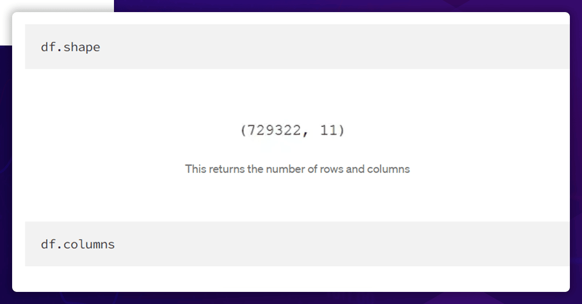
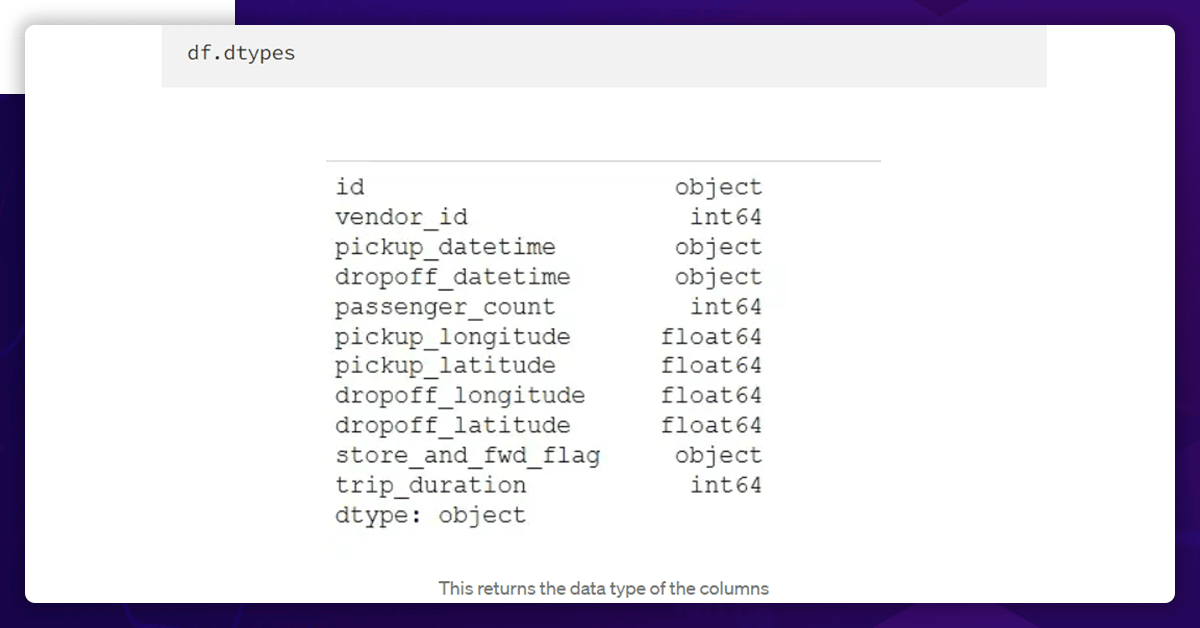
We will examine the shape, columns, column data types, and the first five rows of the data after reading the dataset into the DataFrame df. Using this method, we will be able to summarize the data quickly.

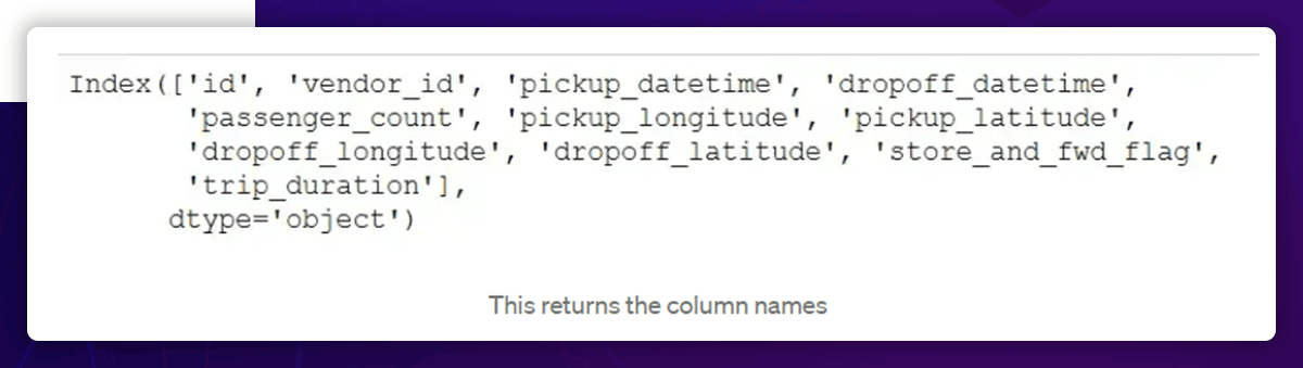
ID: a unique identifier for each journey

Vendor_id: It is a code that identifies the service provider connected to the trip record.

Passenger count: The total number of people riding in the car (driver entered value)

Trip Details Data

Pickup_Longitude: The date and time at which the meter was busy

Pickup_latitude: The time and date at which the meter was not working.

Dropoff_longitude: the latitude at which the meter stopped working

Dropoff_latitude: the location where the meter was not working.

store_and_fwd_flag:

The store_and_fwd_flag determines if the record was saved before delivering it to the vendor. Because the vehicle might sometimes lose the service connection (Y=store and forward; N = not a store and forward trip

Trip duration: The intended length of the journey in seconds

As a result, our data set consists of 11 columns and 729322 rows. There are ten features and the trip duration target variable.

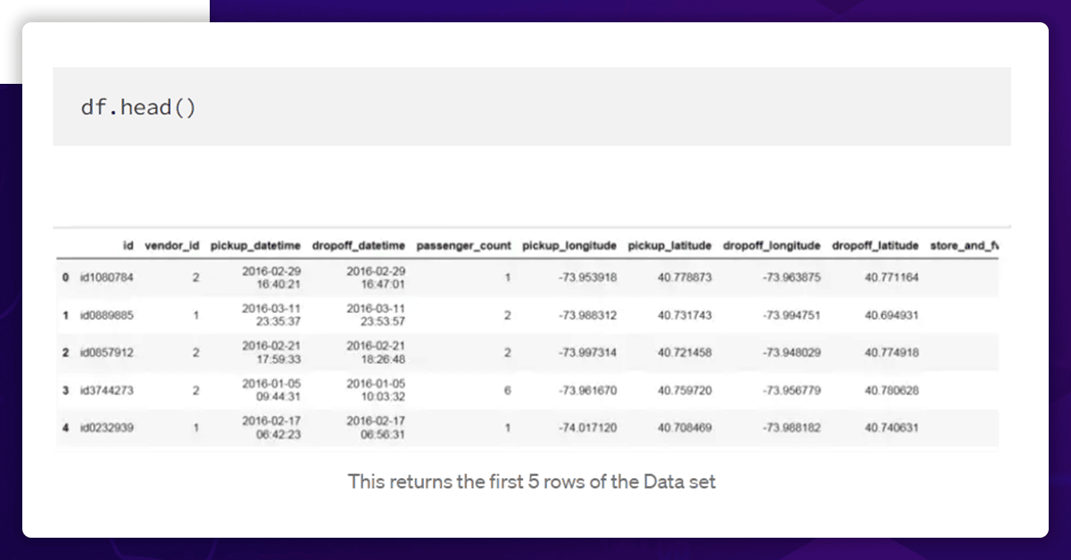
Thus, by examining the first five rows returned by df.head, we may acquire an overview of the data set (). It is possible to specify the number of rows to return by passing it as a parameter to the head () function.

Observations regarding the data

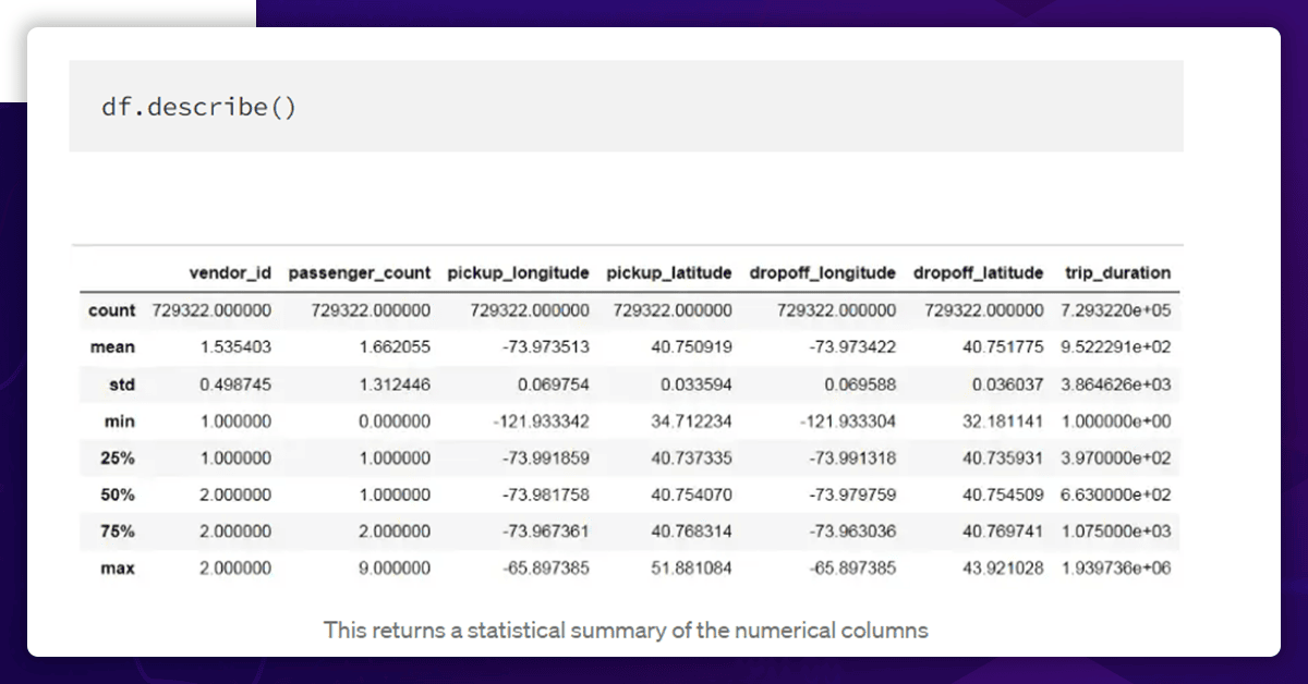
The returned table provides the following details:

Let's quickly review the columns that do not include a number.

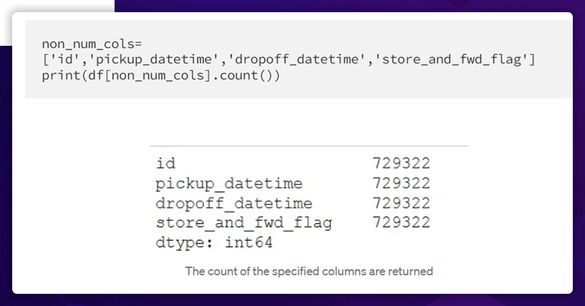
The non-numerical columns also have all the values.

Since the two columns, pickup_datetime and dropoff_datetime, are in datetime format. It is much simpler to analyze time and date data.

Using a Single Variable

Analyze the distribution of variables in the data set

Passenger Numbers

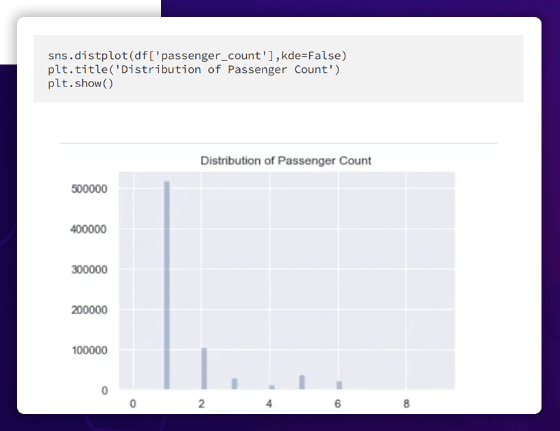
There are typically only 1 or 2 passengers using the taxi. Large groups of people traveling together are unusual.

The Allocation of the Week's Pickup and Dropoff Days

The values received were 709359 and 709308. These two columns illustrate the wide range of pickup and dropoff dates.

It is preferable to convert these dates into days of the week to discover a pattern.

Now, check the distribution of weekdays.

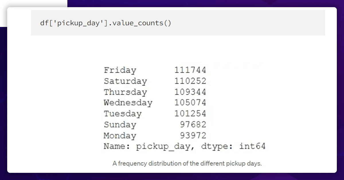
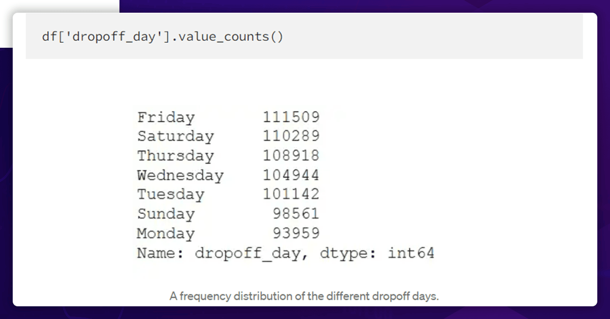
Thus, Fridays and Mondays were the days with the least number of trips. It is also important to consider how the length of the trip varies depending on the day of the week.

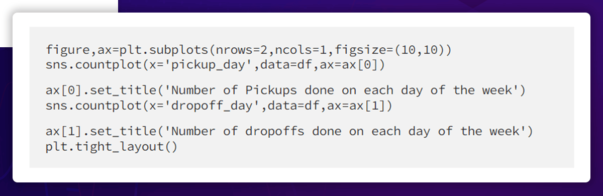
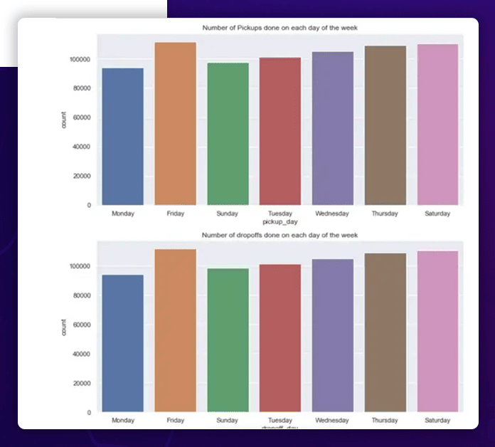
Graphical representations of the distribution of weekdays are also possible.

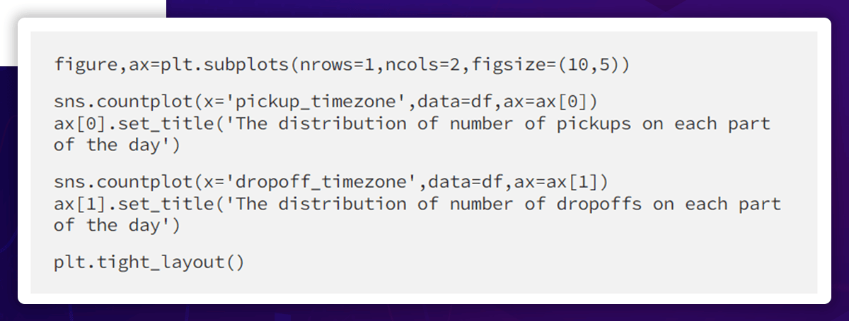
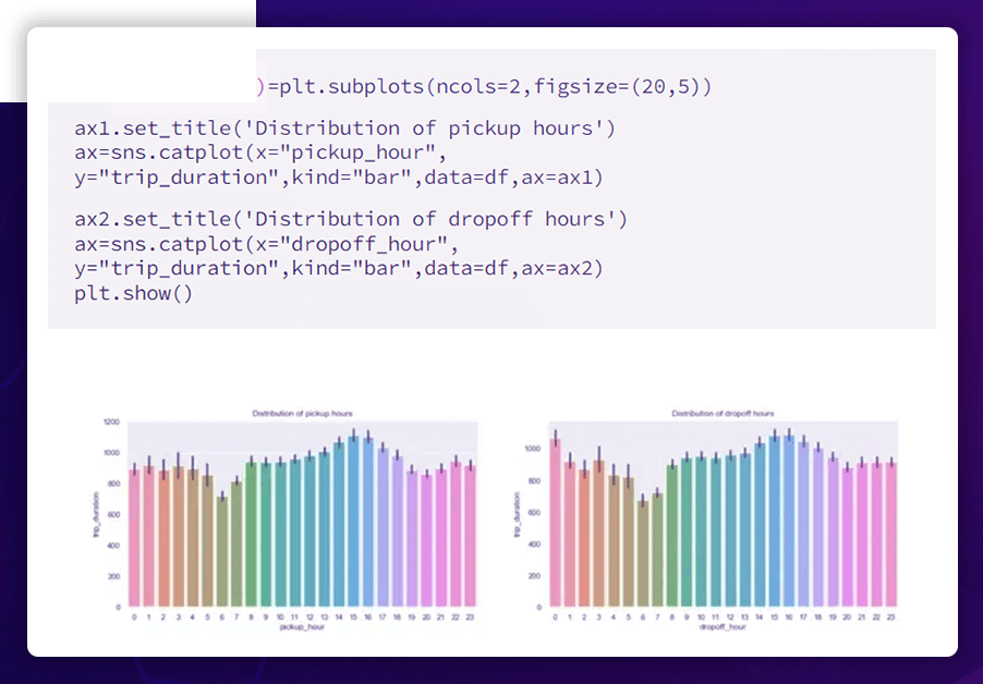
The breakdown of pickup and dropoff times during the day

You can use Hours, minutes, and seconds to describe the time, which makes analysis difficult. As a result, we divide the time into four time zones: morning (4 to 10 hours), midday (10 to 16 hours), evening (16 to 22 hours), and late night (22 hrs to 4 hrs).

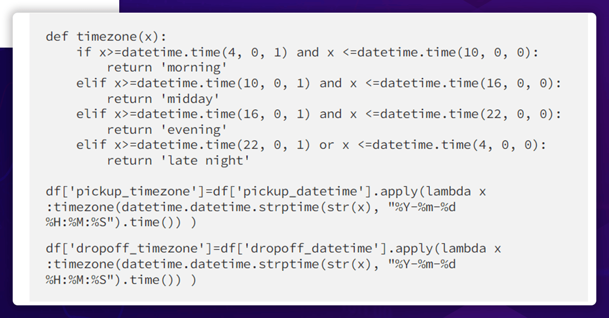
Check the distribution of the Time zone.

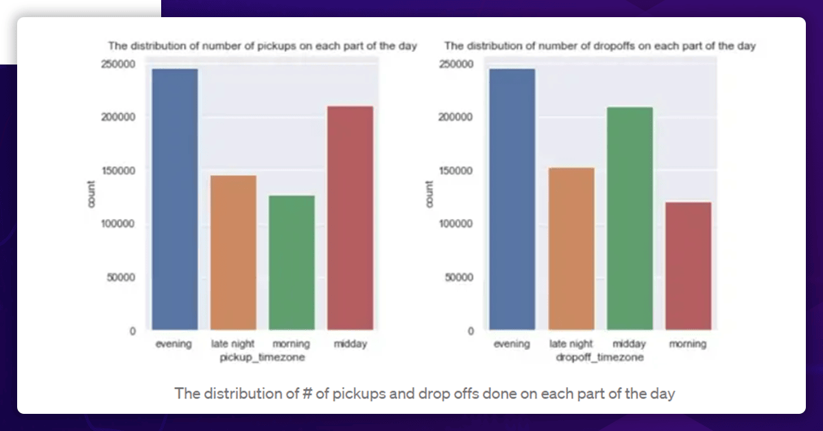
Thus, we see that most pickups and drops occur in the evenings. At the same time, fewer pickups and drops occur in the morning.

Add another column showing the time of the day for pickup.

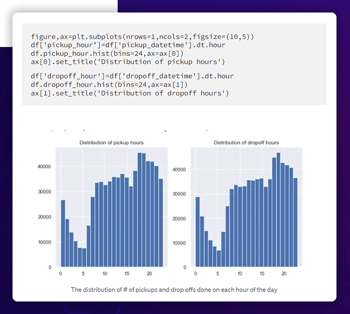
The two distributions are practically identical and line up with how the hrs. of the day were previously split into four sections and distributed.

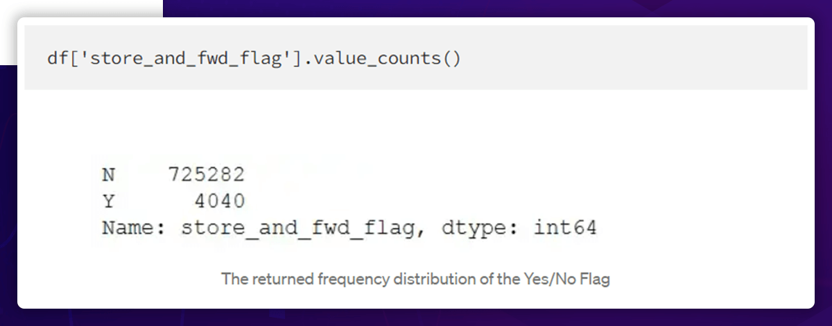
Stored Flag and Forward Flag Distribution

Trip Duration Distribution

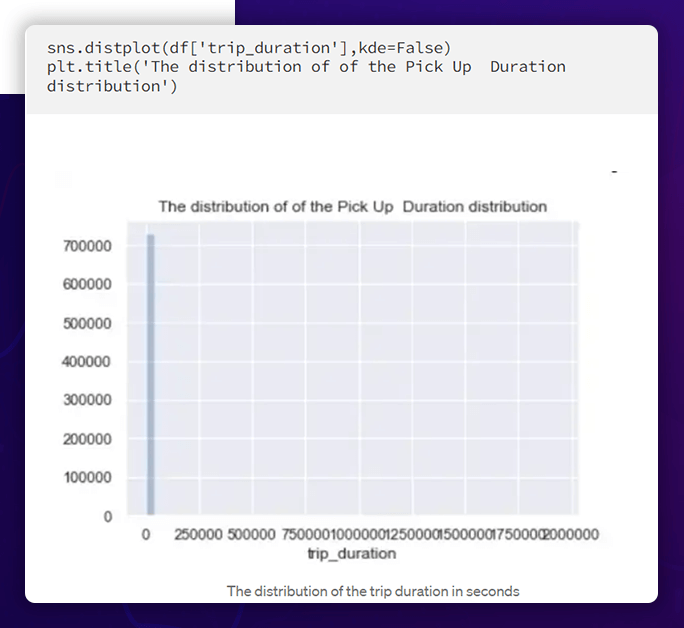
Outliers are present because of the solid right skewness in this histogram. Let's look at this variable's boxplot.

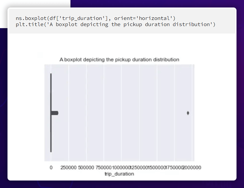
As a result, we can see that there is only one value close to 2000000, while all the others fall between 0 and 100000. There will be a need to handle a value close to 2000000.

Let's look at the top 10 values for trip duration.

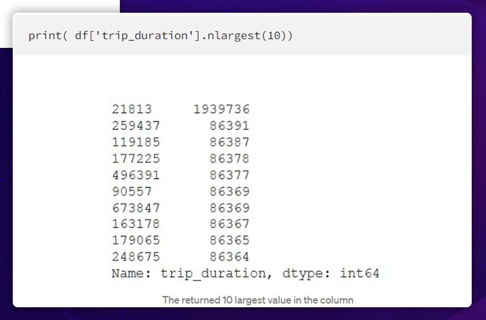
The most outstanding figure is significantly larger than the second and third largest values for journey duration. Data collection errors may result in this, or the data may be accurate. It is best to remove this row before further investigation because the occurrence of such a significant value is unlikely.

It is also possible to replace the value with the mode or median of the journey duration.

Check the trip_duration distribution after the removal of the outlier.

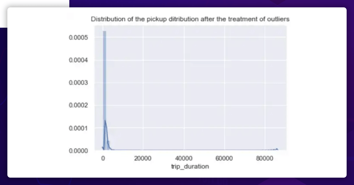
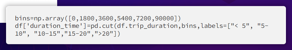
There is still a strong right skewness. So, we will set up an interval within the trip duration column.

As determined by the following:

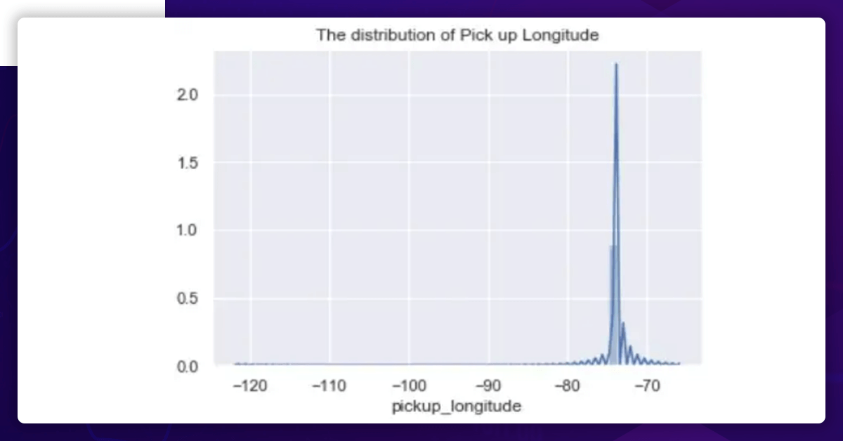
Pickup Longitude Distribution

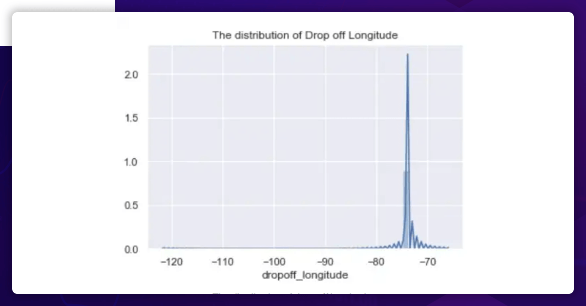
DropOff Longitude Distribution

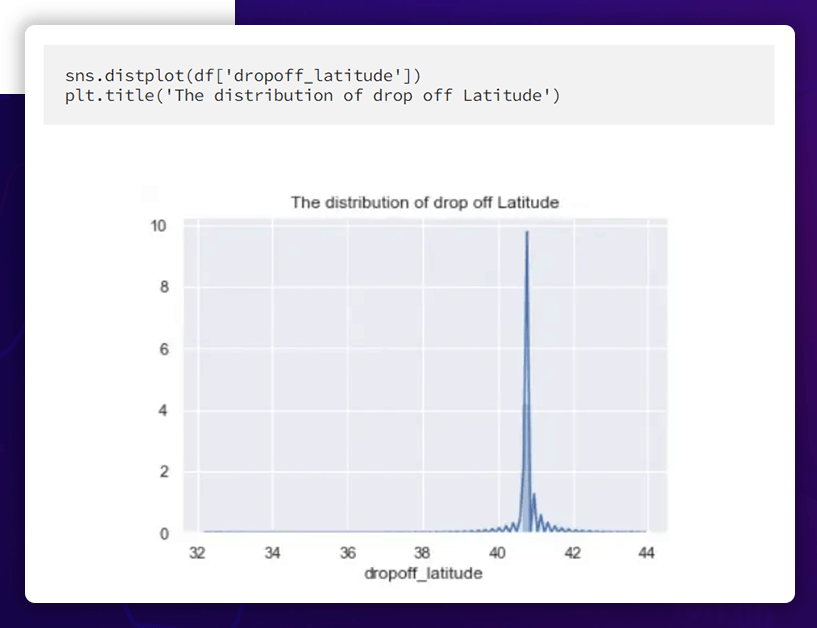
DropOff Latitude Distribution

Pickup Latitude Distribution

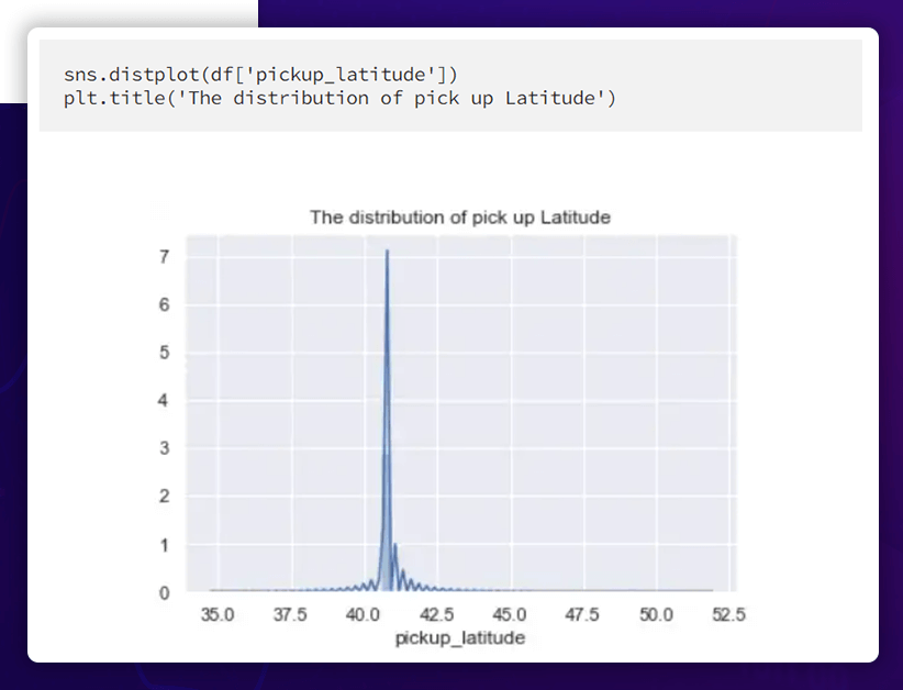
While the pickup latitude and the dropoff latitude have somewhat different distributions, the pickup longitude and the dropoff longitude have practically the same distribution.

Vendor_Id Distribution

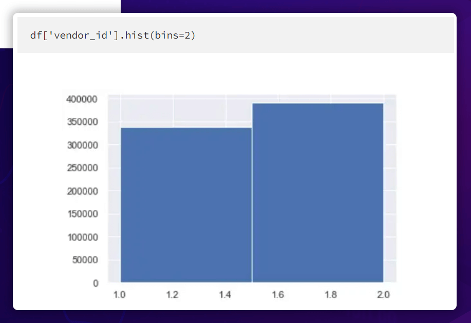
Vendor ID distribution is much in line with expectations.

Analysis of Variance

Let's examine how each variable interacts with the goal variable, trip duration.

Relationship between Day of the Week and Trip Length

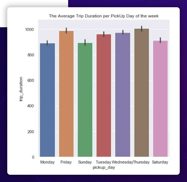
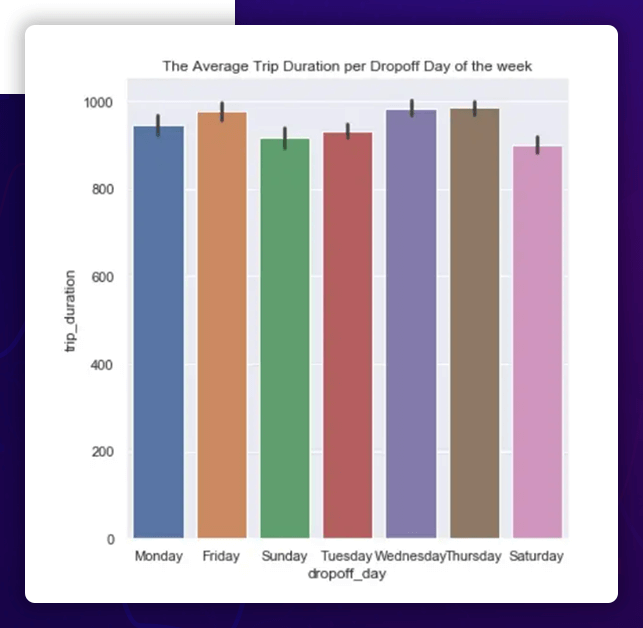
As a result, Thursday has the longest average time necessary to complete a journey, while Monday, Saturday, and Sunday have the lowest average times.

It is still necessary to do more. In addition, consider the consumption of how many short, medium, and long excursions each day.

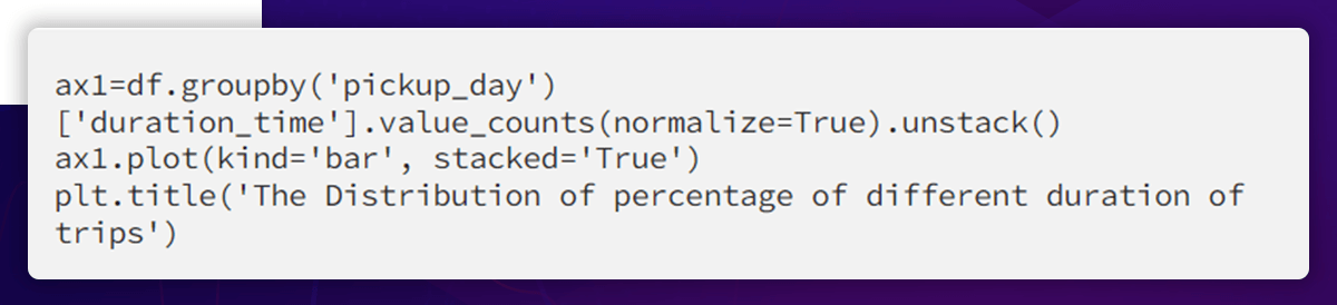
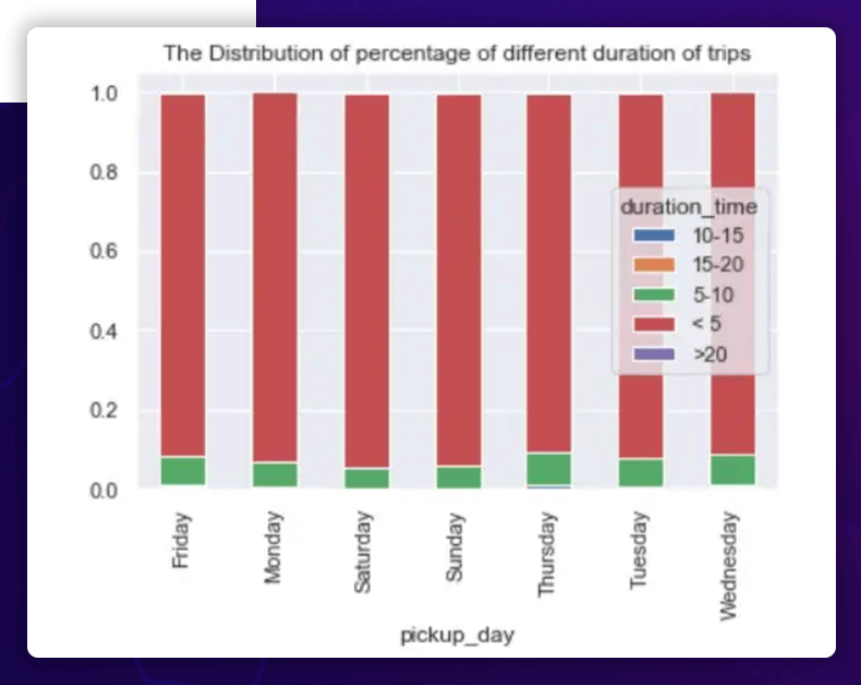
There are more daily travels between 0 and 5 hours, so this only provides a few insights.

Examine the percentage of just lengthier trips (those lasting more than five hours).

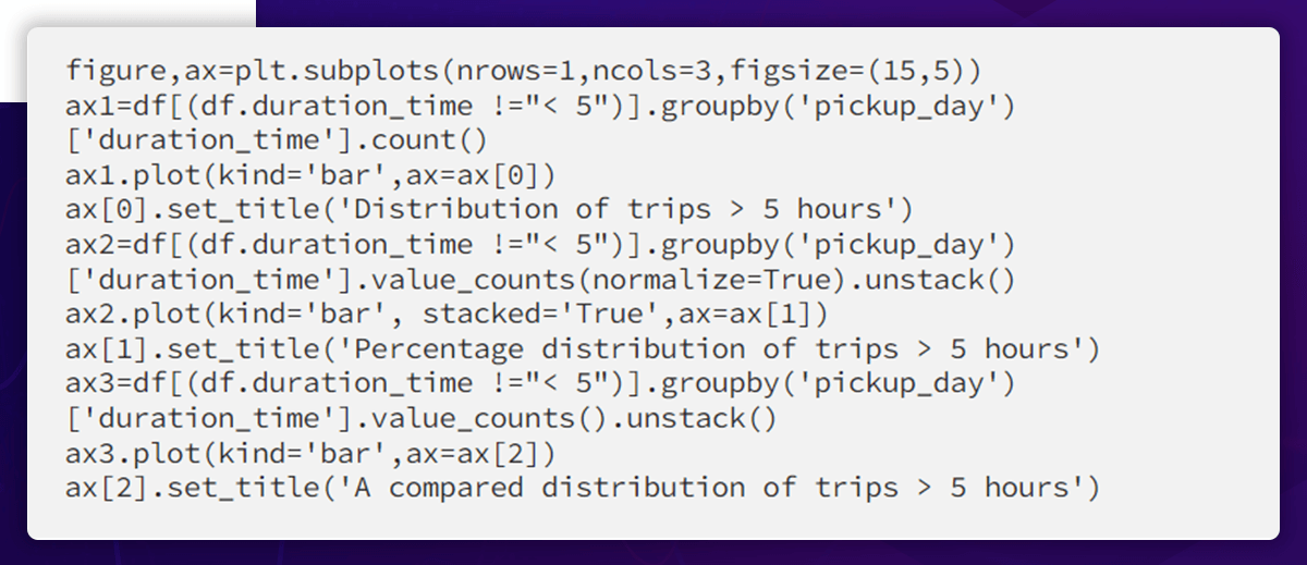
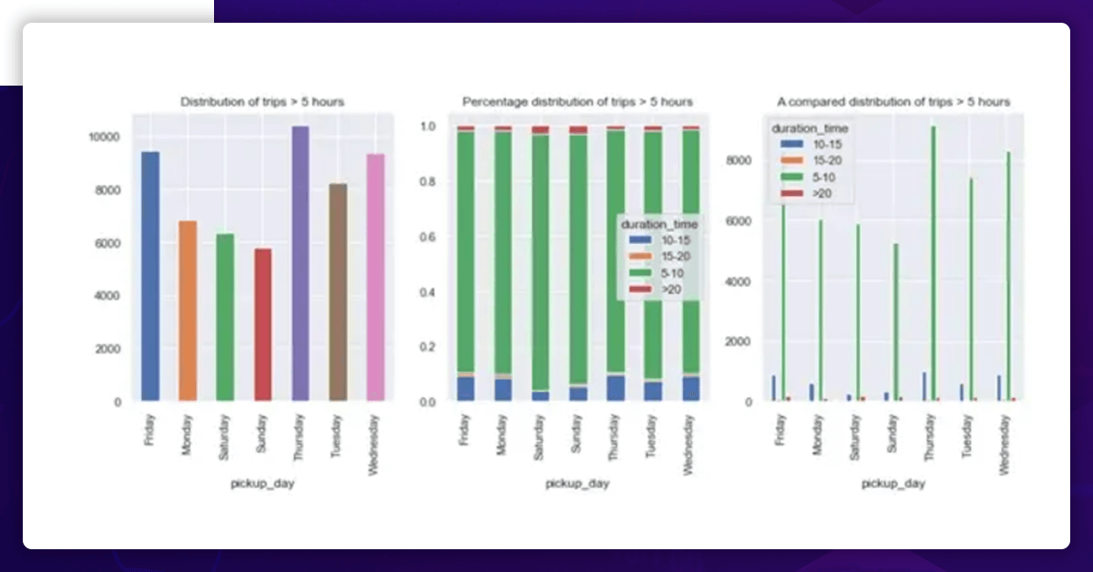
Here, the three graphs display three different sorts of data:

Important things include:

Thursday saw the highest number of trips lasting more than five hours, followed by Friday and Wednesday.

Thursday saw the most journeys of 5 to 10 minutes and 10-15 minutes (see left graph).

But there are more excursions lasting for more than 20 hours on Sunday and Saturday (right graph).

(Center Graph)

The Connection Between Trip Length and Time of Day

The average length of time necessary to finish a trip is highest for noon travels (between 14 and 17 hours) and lowest for early morning trips (between 6–7 hours)

The Relation of Number of Passenger and Duration

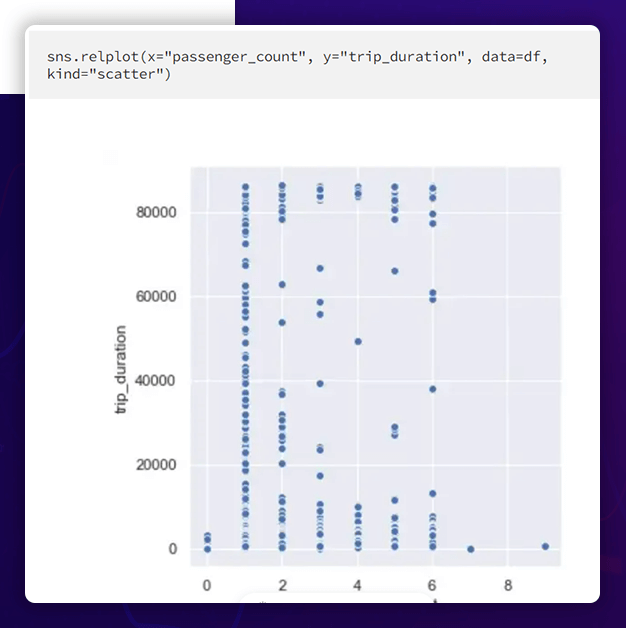
As can be seen, the number of passengers and the length of the trip do not correlate. However, one should highlight that seven or nine-passenger counts do not take longer trips. Only for passenger count 1, however, is the travel time roughly divided evenly.

The Connection Between the Vendor ID and the Duration

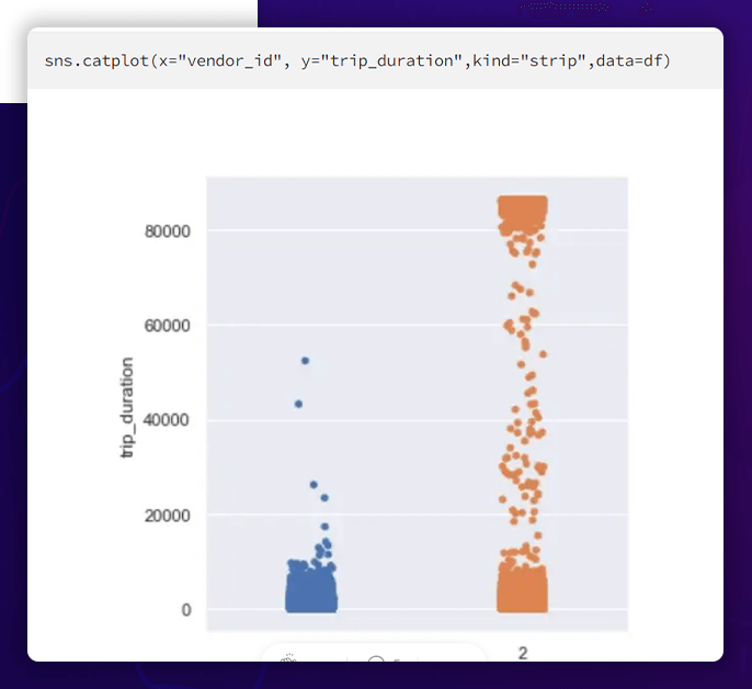
Here, we can observe that seller one mainly offers short journeys, whereas vendor two offers both short and long excursions.

The Correlation Between the Duration and the Store Forward Flag

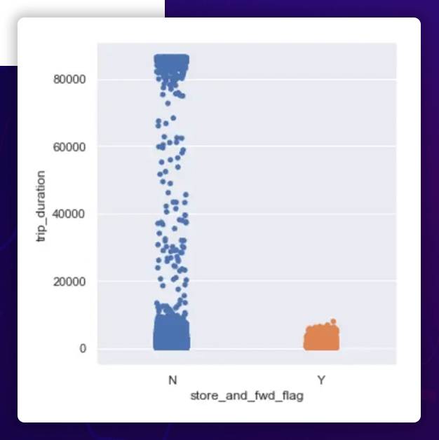
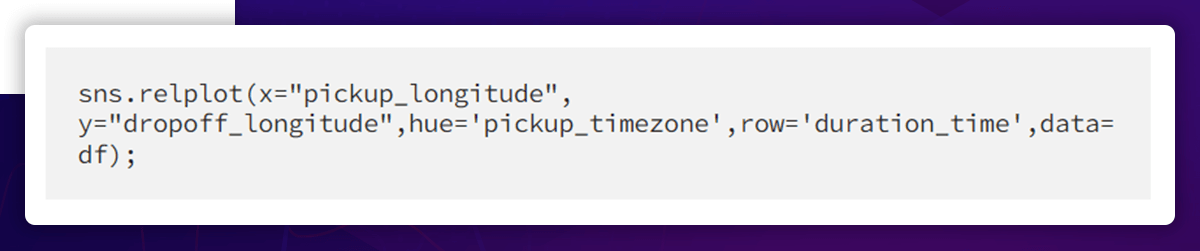
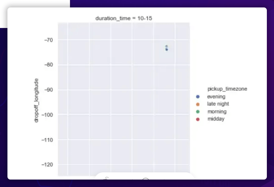
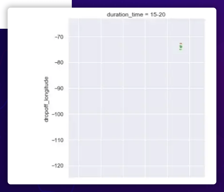
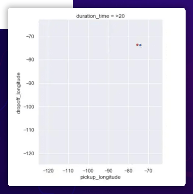
The correlation between the Geographical Location and Duration

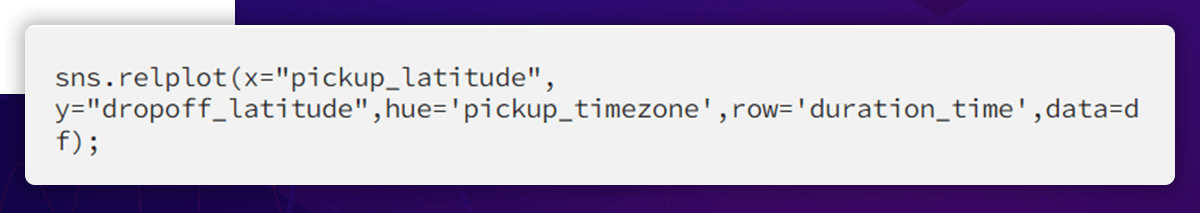
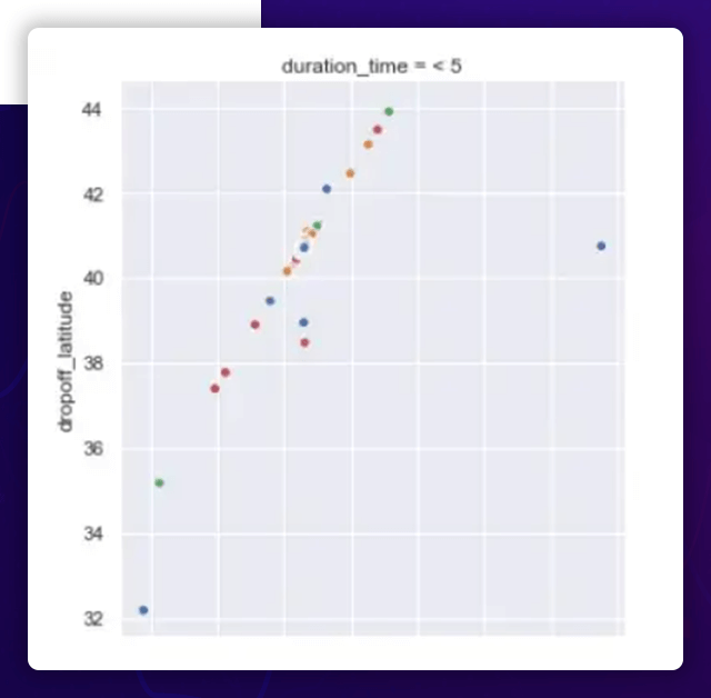
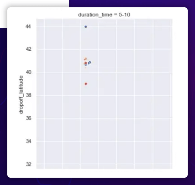
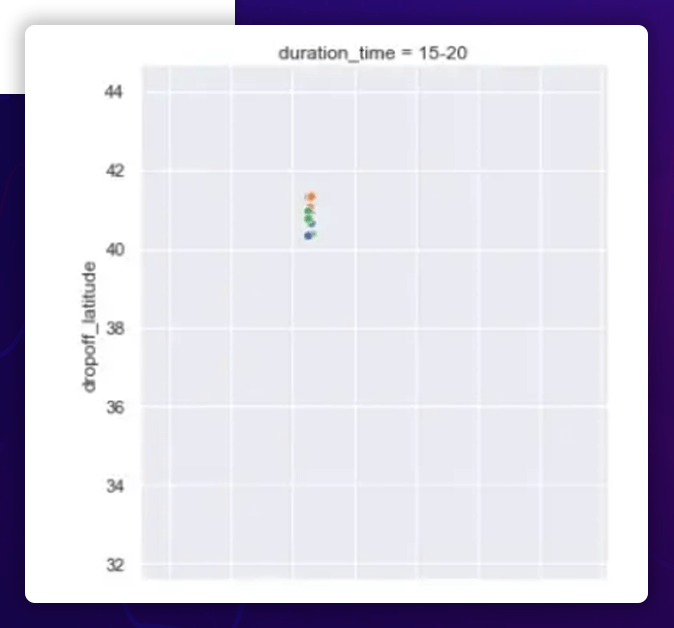
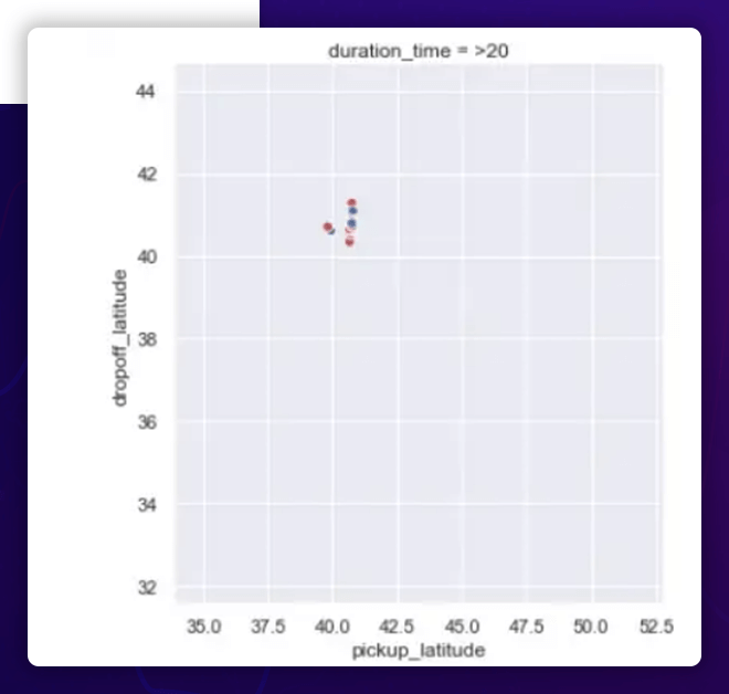
Observation

The pickup and dropoff latitudes are more or less uniformly spread between 30 ° and 40 ° for shorter excursions (5 hours) and between 30 ° and 40 ° for longer trips (>5 hours). The entire pickup and dropoff latitude range from 40 to 42 degrees.

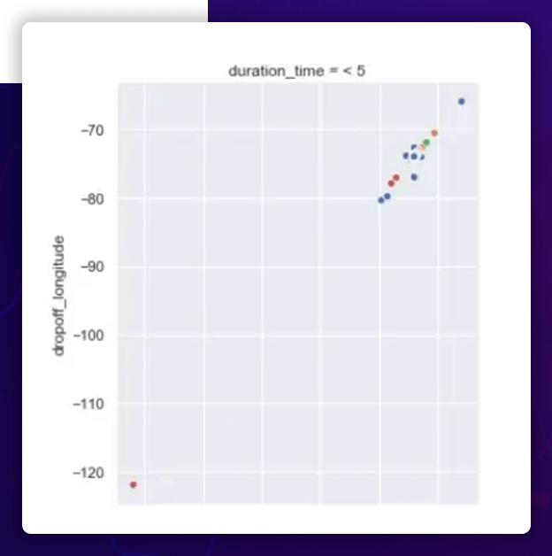
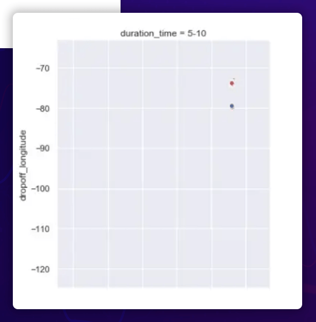
Observation

Data Set and Trip Duration Conclusion:

Conclusion

So, you can see how web scraping services and exploratory data analysis aids in finding underlying trends in the data, enables us to make inferences, and even forms the basis for feature engineering before starting to create our model.

If you are looking to fetch exploratory data analysis on taxi trip duration dataset for any country, then contact Web Screen Scraping today!

Request for a quote!